
Crime Trends in Canada
Its not that bad, but the data could be better.

Data
The latest Uniform Crime Reporting Survey released on July 22nd 2026, several tables are generated from this data :
Table 35–10–0026, Crime Severity Index and weighted clearance rates by census metropolitan area (CMA). Raw incident counts treat a shoplifting charge and a homicide as equally weighted events. The Severity Index corrects for that by weighting each offense by its average sentence, so it measures how serious the crime picture is, not just how busy police are.
Table 35–10–0177 , incident-based crime statistics by census metropolitan area
Table 35–10–0071, homicide victims by CMA. Homicide is tracked on its own because it is rare, well defined, and reliably reported. It isn’t affected by the classification and reporting-behavior issues that complicate other categories, which makes it one of the most trustworthy indicators in the dataset.
Also Table 35–10–0164 tracks self-reported violent victimization that was reported to police, from the General Social Survey on Victimization. It’s the only measure here that captures crime that happened but was never reported to police at all. The catch is that this survey only runs occasionally, roughly every five years, while the incident-based tables above update annually. we will not be looking more at this here but we do hope it gets updated soon.
Getting and using the data :
I have an perpetually under development repo, I use to look at statscan data on github called cansimr.
dat <- cansim_get(’35-10-0177’)
md = attr(dat, ‘metadata’)
Which will obtain me that tables data and metadata.
Approach
Filter the data for legacy violations like:
Total prostitution [320]
Sexual offence which occurred prior to January 4, 1983 [1300]
Filter also for just the leaf nodes of the hierarchical geographical area and Normalize both the yearly data and the value data, which is reported crime per 100,000 people
dat |>
mutate(ref_date_norm = (ref_date - min(ref_date) ) / (max(ref_date) - min(ref_date))) |>
mutate(value_log = log(value + epsilon)) |>
mutate(value_norm = (value - mean(value))/sd(value), .by = violations)
Make sure to remove any data for a crime before the first violation is recorded and the next several years due to ramp up effects in law enforcement.
dat_trends_valid <-
  dat_trends_selected_violations |>

  # Remove years before first offence
  mutate(first_valid_year = min(ref_date[value > 0]), .by = violations) |>
  filter(ref_date > first_valid_year) |>

  # Remove years after last offence
  mutate(last_valid_year = max(ref_date[value > 0]), .by = violations) |>
  filter(ref_date <= last_valid_year) |>

  # Ramp-up trim: only for violations introduced AFTER the panel start,
  # drop the 5 years following introduction to let reporting coverage stabilize
  mutate(is_new_code = first_valid_year > panel_start + 1) |>   # +1 year buffer for edge cases
  filter(!is_new_code | ref_date > first_valid_year + 5) |># +5 year buffer for police ramp up
  dplyr::select(-first_valid_year, -last_valid_year, -is_new_code) |>

  # Re-check minimum series length AFTER the ramp-up trim
  mutate(n_years = n_distinct(ref_date), .by = violations) |>
  filter(n_years >= 15)
Split into two approaches (many small models):
Create a simple linear model for each combination of geographic area and violation and look for cities where the slope seems to be increasing in all case.
  city_slopes <-
    dat_trends_valid |>
    ####################
    # Remove slopes with less then 8 datapoints
    mutate(n_obs = n(), .by = c(violations, geo)) |>
    filter(n_obs >= 8) |>
    summarize(
      slope = tryCatch(
        stats::coef(stats::lm(value_norm ~ ref_date_norm))[[”ref_date_norm”]],
        error = function(e) NA_real_
      ),
      .by = c(violations, geo)
    )
consistency <-
  city_slopes |>
  summarize(
    n_cities = n(),
    slope_mean = mean(slope),
    slope_sd = sd(slope),
    pct_positive = mean(slope > 0),
    .by = violations
  ) |>
  arrange(desc(pct_positive))
this simple idea gives us an check on if our other technique is working.
> consistency |> arrange(desc(pct_positive))
# A tibble: 39 × 5
   violations                       n_cities slope_mean slope_sd pct_positive
   <glue>                              <int>      <dbl>    <dbl>        <dbl>
 1 Extortion [1620]                       36      2.14     1.84         1
 2 Total sexual violations against…       36      2.30     0.964        1
 3 Child Sexual Abuse and Exploita…       36      1.58     1.50         0.972
 4 Sexual assault, level 1 [1330]         36      1.19     1.77         0.833
 5 Total firearms, use of, dischar…       36      1.22     1.29         0.833
 6 Total other violent violations …       36      0.391    3.72         0.833
 7 Fraud [2160]                           36      1.19     1.75         0.806
 8 Sexual assault, level 2, weapon…       36      0.816    1.09         0.778
 9 Assault, level 2, weapon or bod…       36      0.960    1.48         0.778
10 Shoplifting $5,000 or under [21…       36      1.09     1.32         0.75
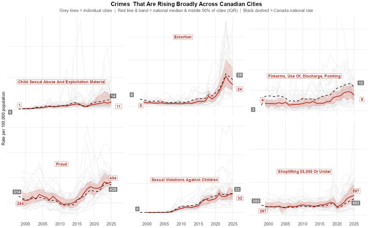
This shows us that Extorition seems to be going up in every canadian city with an average slope of 2.14.
Split into two approaches (two - a single larger model):
fit <- lme4::lmer(
 value_norm ~ ref_date_norm + (1 | geo) + (1 + ref_date_norm || violations)
  data = dat_trends_valid
)
With a fixed effect on ref_date_norm estimates (-0.2429) the relation between time and the normalized number of reported offences per 100,000 population. both are normalized of course as above. But over all the value goes down.
Random Intercept (1 | geo) each CMA gets its own starting level but they will share the same trend over time
Uncorrelated Random Intercept & slope (1 + ref_date_norm || violations). Allows each of the selected violations types to have its own baseline starting value, and have its own unique trajectory over time. the double pipe makes the correlation between a violation’s starting point and its slope over time to be zero.
Extracting results
We use merTools::REsim to simulate the random effects and also extract the fixed effects slop (-0.242…)
Then From the simulation of the Random effects we extract the slopes over time for each violation, and estimate the upper and lower bound of each slope.
# Simmulate
resims <- merTools::REsim(fit_uncorr, n.sims = 2000)

# fixed effect slope & its SE (-0.2429019)
fe_slope <- lme4::fixef(fit_uncorr)[”ref_date_norm”]

# Filter explicitly by group and term name
national_trend <-
  resims |>
  filter(
      groupFctr == “violations”,
      term == “ref_date_norm”
  ) |>
  transmute(
    violations = groupID,

    # Add overall fixed slope to individual random slope shifts
    est    = mean + fe_slope,
    lwr_95 = (mean - 1.96 * sd) + fe_slope,
    upr_95 = (mean + 1.96 * sd) + fe_slope
  ) |>
  tibble()
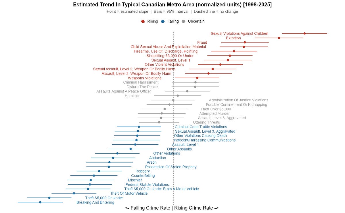
We now have all the data we need in a dataframe called national_trend. checking this we see that these all appear in the list above, so broadly both techniques are getting us to a similar spot.
> national_trend |> arrange(desc(lwr_95)) |> head(5)
# A tibble: 5 × 4
  violations                                                                      est lwr_95 upr_95
  <chr>                                                                         <dbl>  <dbl>  <dbl>
1 Total sexual violations against children [130]                                 2.38  1.97    2.79
2 Extortion [1620]                                                               1.91  1.47    2.35
3 Fraud [2160]                                                                   1.30  0.862   1.73
4 Child Sexual Abuse and Exploitation Material (Possessing or Accessing) [3455]  1.28  0.841   1.71
5 Total firearms, use of, discharge, pointing [150]
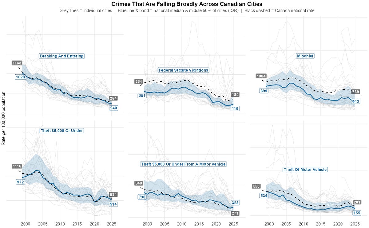
But not all crimes are going up, some crimes are going down.
> ##############
+ # Crimes that are going down in many places?
+ national_trend |> arrange(upr_95) |> head(5)
# A tibble: 5 × 4
  violations                                          est lwr_95 upr_95
  <chr>                                             <dbl>  <dbl>  <dbl>
1 Total breaking and entering [210]                 -2.41  -2.82  -2.01
2 Theft $5,000 or under [2140]                      -2.25  -2.65  -1.85
3 Total theft of motor vehicle [220]                -1.80  -2.21  -1.39
4 Theft $5,000 or under from a motor vehicle [2142] -1.55  -1.95  -1.14
5 Total Federal Statute violations [400]            -1.51  -1.91  -1.11
Plotting Results we see, some crimes are rising and some are falling.
We can also look at the top few and see how they are changing over time in more detail.
A tale of 34 Cities
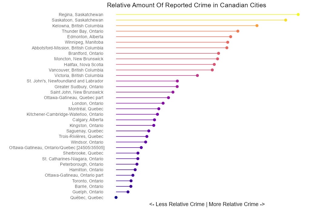
We can also see how this crime expresses it self in different cities
# Extract city baseline levels
city_levels <-
  resims %>%
  filter(groupFctr == "geo", term == "(Intercept)") %>%
  transmute(
    geo    = groupID,
    # Overall fixed intercept + city random intercept offset
    est    = mean + fe_intercept,
    lwr_95 = (mean - 1.96 * sd) + fe_intercept,
    upr_95 = (mean + 1.96 * sd) + fe_intercept
  ) %>%
  inner_join(
    geo_years  |> filter(n_years_with_data >=15),
    by = 'geo'
  ) |>
  arrange(desc(lwr_95))
Making a lollipop plot of the data we see some cities like Regina and Thunder Bay have relatively higher crime rates while cities like Guelph and Quebec City have a lower relative crime rate.
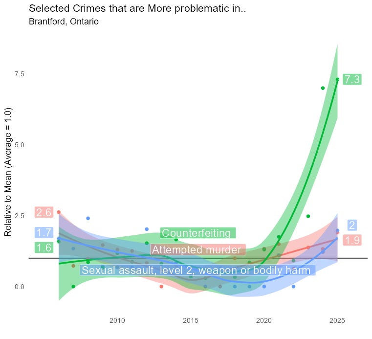
But we can go further, while some crimes Go up or down with nation wide trends, some are local phenomenon. looking at the three top crimes in some of the more problematic cities in Canada.
Winnipeg
We see that Winnipeg has five times the robberies of a typical Canadian City.
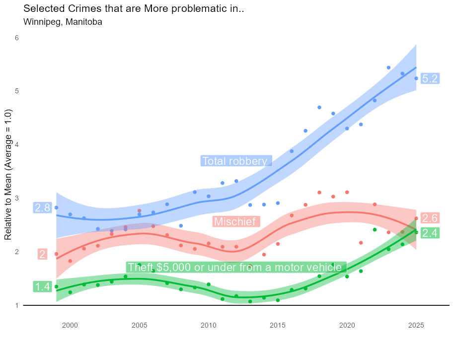
Posting some of this data on Reddit, led to a lively discussion with many deriding the large pay of the police in the city
Regina
We see that Regina has 7 times the amount of Arson, 4 times the amount of attempted murder relative to average city.
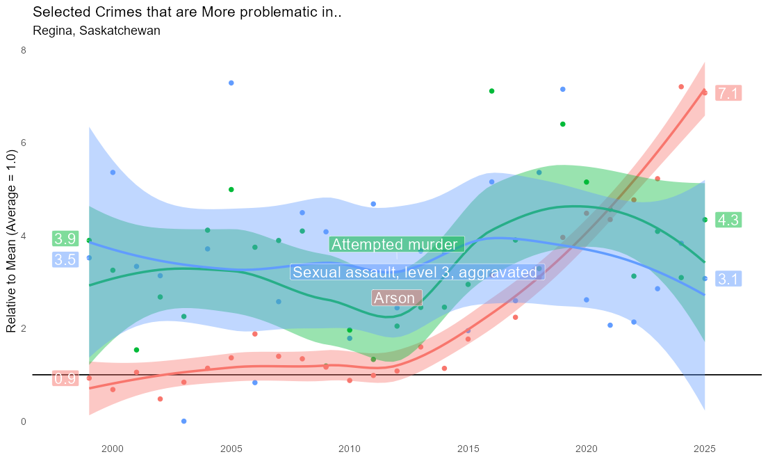
The discussion of this data on reddit also led to a lot of talk about police budgets. But, it did seem that in this case there was a variety of opinions about the size of the budget.
Thunder Bay
Thunder Bay (The murder Capital of Canada) also has robbery and and shoplifting reports above the typical Canadian city.
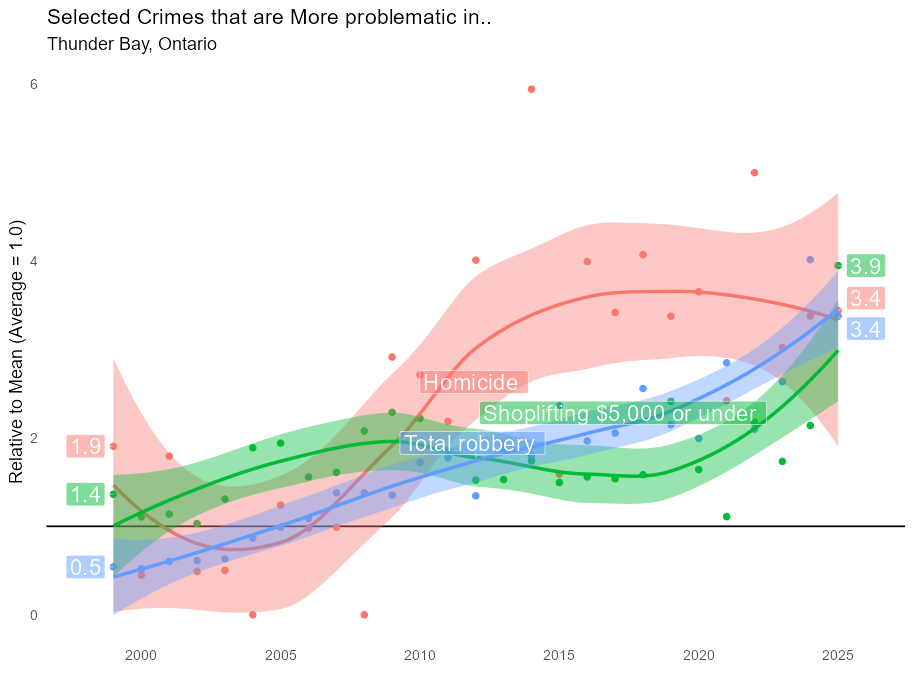
I felt the reddit discussion in Thunder bay was particularly informative, with many users citing specific streets and buildings of well known illegal activity and gang houses, with some speculating of the reasons these known spots were allowed to continue opperating.
Brantford
While Brantford seems to have more reports of Counterfeiting then any other city by far. And this seems to be a very recent trend.
Final Thought
Some types of Crime are going up, Some are going down. Some Crime follows a national trend and might be better looked that way. While some crimes are likely local phenomenon, and should be tackled locally.
Also in General I did not do Inter country comparison, but my suspicion is that Canada is pretty safe overall.